
Lesson 1 - Introduction To Microsoft Excel and Google Sheets
A Process and Workflow Design Training Series...
Mastering Microsoft Excel and Google Sheets
If you’re an accountant or bookkeeper and you don’t feel like you’ve mastered Excel and Google Sheets... this course is for you!
Spreadsheets have been around since the 1960s. The very first spreadsheet was called “Visicalc” and it looked like this:

Then there was Lotus 1-2-3...
Then Quatro Pro...
Then Microsoft came out with Excel and for a long time it was game over for all other spreadsheets.
Until Google Sheets came along.
Now It’s Game On!
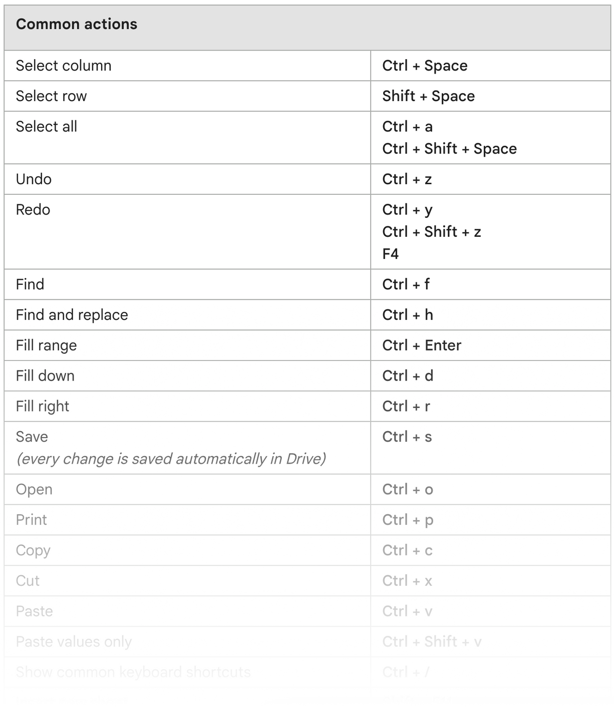
Let’s start with some keyboard shortcuts. If you take the time to learn these, and at first you have to force yourself a bit to use them, they will become second nature and you will fly around a spreadsheet at just about the speed of thought.
In other words, as quickly as you can think of something, you can do it without taking your hands off the keyboard.
In this lesson’s exercise file you’re going to learn your way around Excel and Google Sheets and we’ll start with a list of common keyboard shortcuts.
If you are using Google Sheets you can enable these legacy Excel keyboard shortcuts by following the instructions here:
Have you ever looked up the definition of the word “Practice?”

I love the first verb definition.
Keyboard Shortcuts
If you use these shortcuts repeatedly (force yourself at first) they will become second nature. And when they become second nature, as quickly as you can think of highlighting a row in Excel or Google Sheets, you'll hit [SHIFT]+[SPACE BAR] and your row will be highlighted.
Then a [CTRL]+[-] will delete that row.
And of course [CTRL]+[SPACE BAR] will highlight any selected columns.
Then a [CTRL]+[-] will delete those columns.
** STOP **
If you just read the above and thought, “oh that’s cool” or, “yeah I know that” and you don’t already do this instinctively when you are working in a spreadsheet, and assuming this time right now while you are reading this is time you’ve set aside to learn this stuff, then stop right now, open up the exercise file or any spreadsheet and practice these shortcuts.

Important Housekeeping Notes on the Exercise Files
If you want to work with the exercise files in Google Sheets, these links take you to a read only copy.
Click File, then Make a copy, and Google Sheets will copy it into your My Drive folder in whichever Google account you are logged into.
If that last sentence made no sense, then get my course called, “Run Your Accounting or Bookkeeping Practice with Google Workspace™” and this will all make a TON of sense.


If you want to work with the exercise files in Excel, Click Here then:
- Choose File
- Then Download
- Then choose Microsoft Excel
The first tab gives you the list of keyboard shortcuts from above.
Practice them. That means do them over and over and over again until they become second nature.
Little Boxes - What’s In A Cell?
A spreadsheet is made up of a whole lot of little boxes called, “Cells” and those cells make up a “worksheet” (tabs), and those worksheets make up a workbook.
When you copy and paste a cell, you take everything with you - the value, the formula (if any), and any formatting you’ve applied. It’s helpful to understand this at the most granular level because there are times when you don’t want to take everything with you. You may only want the value, or the formula, or the formatting.
Using your copy and paste special commands you can see the various components of your cells.
In the exercise file from this lesson, open the tab called, “Seth’s Scrap Sheet” and you will find a few cells with different kinds of information in them.
Highlight any or all of the cells and press [CTRL]+C to copy, then right click and choose “Paste Special.” Up to this point it works exactly the same in either Excel or Google Sheets.


If you paste the formatting it will apply any number format, like percent or comma formatted, as well as any fill and font color and any borders. These are all part of the “formatting.” If you paste the value, you will get none of the formatting and if there is a formula, you will wind up with just the value resulting from that formula at the moment you copied it.
Excel has a really nice feature here in terms of the operations. I use ‘Multiply’ frequently when I need to convert positive numbers into negative, by copying a “-1” and then I paste, special, multiply across the range of numbers.
To accomplish this in Google Sheets you would have to perform a few steps, to multiply the range by “-1” and then past the values of that back onto the original range.
Another common use case for Paste Special is to convert a series of cells containing formulas into hard numbers.
You copy the range, and without clicking away (ie the same range is still selected) you past the values right back onto that same range. This will replace all of the formulas with their results.
In the exercise file I’ve given you examples of different kinds of data and formatting. You won’t see it until you look at the contents of the cell, but cell C5 contains a formula.
Practice this until it becomes second nature. Then make a conscious effort to look for opportunities to use these tools in your every day work. This is how I have mastered this stuff. By using it as much as possible.
NAVIGATION
The second tab is the “Navigation Practice Sheet.” Click on that.
This is just a simple sample budget, but the point is not the information itself. It’s the layout. In this exercise I want you to practice moving around the data quickly.
Start on cell A1. If you are not there, press [CTRL]+[Home]
Press [CTRL]+[Right Arrow].
It stops you on “Item / Category” because you started on a blank cell and immediately hit one that had something in it.
Do it again.
It stops you on Dec because you started on a cell with something in it, so it goes across the range until it sees a blank and it stops on the last cell with something in it.
Now move down.
Once gets you to the $625 (assuming you haven’t changed the number).
Again gets you to the last number.
One more time gets you to the total.
Practice moving around this data. It’s a bit like playing a video game. Once you get used to the controls you start getting faster and faster at maneuvering your cell pointer and getting around a spreadsheet quickly.
In this case it might not seem significant, but when you have a large spreadsheet with lots of data these kinds of maneuvers can save you a lot of scrolling.
WORKING WITH BANKING DATA
File Management
Here’s a PDF of one of my bank statements from December 2018.
Using MoneyThumb’s PDF2csv I am able to convert this beautifully and in seconds to a csv file, which can be opened in Excel.
I like converting these to csv’s instead of importing directly into QBO for two main reasons.
First, the csv file may be useful for other purposes so I like to have the file on record.
Second, as you’ll see next, we want to manipulate the data before importing it.
If you are using Google Sheets, presumably you will have Drive for Desktop installed. This allows you to browse your files in File Explorer (Windows) or Finder (Mac).
With the converted csv file in a google drive folder you can access that file on the web and open it in Google Sheets. Or you can open it from Google Sheets from within File Explorer as explained below.


These are the same folder, one is streamed (not mapped) locally and the other is on the web.
In the local folder you can double click it, and it will open in Excel.
If you want to open the file in Google Sheets, you can either go to the folder on the web (browser), or right click in File Explorer and open it in Google Drive.

A preview will open in your browser. Then you can open it with Google Sheets:

This may seem a bit drawn out, but in reality it’s a couple of clicks and in less than 30 seconds you have it in Google Sheets. You will see this demonstrated in the live session or the recording. And now the file is open in an environment where it is ridiculously easy to share and collaborate. To do this with the Excel file, you’ll need to copy it into a Sharepoint folder that is shared with others who are logged into the same account. With google sheets I can invite anyone with just their email address, and that email address just needs to be associated with their own Google or Gmail account.
A CSV file is a generic file type who’s format lends itself easily to be opened in Excel or Google Sheets, but it is devoid of any formatting and it can only contain a single tab.
If you opened the file in Excel, one of the first things you want to do is save it as an Excel file so you don’t lose any changes that aren’t compatible with a csv file.

These basic file operations probably seem elementary to a lot of you, but knowing how to manage these files and file types so well that it’s second nature will make you a much more effective “Master” in creating and manipulating spreadsheets.
Formatting a Bank Statement Download
Open up your Wells Fargo 3051 2018-12-31.csv file. If you are using Excel, save it as an Excel file. If you’re in Google Sheets, once it’s open in Google Sheets, you’re all set.
Let’s format the dates in mm/dd/yy format. This way they will always line up nicely whether it’s within the first 9 days, or later.
Microsoft Excel
Select the range of dates:
Start at cell A2 then press [CTRL]+[SHIFT]+[Down Arrow]
Then press [CTRL]+1
Note - you have to use the number 1 on the top of your keyboard. If you have a number pad on your right, that one won’t work.
CTRL+1 brings up your format cells dialogue. You should be in the ‘Number’ tab, but if not, click on that.
Then choose ‘Date’ and select the appropriate format

Google Sheets
Select the range of dates:
Start at cell A2 then press [CTRL]+[SHIFT]+[Down Arrow]
Then press [CTRL]+1
Note - you have to use the number 1 on the top of your keyboard. If you have a number pad on your right, that one won’t work.
CTRL+1 brings up your format cells menu.
Depending on what you may have done recently in Google Sheets, you might find what you want there as a Date format. If not, click ‘Custom number format’

Then you can type the format you want in there very easily as follows:

Next, format the currency columns according to your preference. Some people like $’s, I personally find them distracting. Also let’s split the view so we can see our headers no matter how far down the spreadsheet we go.
Microsoft Excel

Google Sheets

Next, notice that we have separate columns for debits and credits. And remember that the banks have this backwards. A debit should increase a bank account in normal accounting terms. In order to simplify this, especially if we want to import this data into QuickBooks Online (or desktop) let’s create a single column for the amount. Deposits should be increases (or positive) and payments should be decreases or negative. This process will look identical in both spreadsheets.
Microsoft Excel
First let’s remove the Balance column. We don’t need it. One thing I will often do before removing something like this, is I will copy the tab so I preserve the data as it was before removing the balance. This makes it easy to get it back if I want it.
Then we’ll insert a column after the Debits column and label it “Amount.”
Then we’ll write a simple formula to get the amount column set up exactly the way we need it.

KEYBOARD SHORTCUT
Click to select the entire column, and then press [CTRL]+- (that’s CTRL and the minus sign)
Next right click and insert a column, and label it “Amount”

KEYBOARD SHORTCUT
Move your cell pointer to any cell in the column where you want to insert (Memo in this case), then press [CTRL]+[SHIFT]+[Spacebar].
This highlights the entire column.
Then press [CTRL]+[SHIFT]+[Plus Sign]
That inserts the column.
Then [CTRL]+[Up Arrow] and you should be in cell E1, ready to label the column “Amount.”

Google Sheets
First let’s remove the Balance column. We don’t need it. One thing I will often do before removing something like this, is I will copy the tab so I preserve the data as it was before removing the balance. This makes it easy to get it back if I want it.
Then we’ll insert a column after the Debits column and label it “Amount.”
Then we’ll write a simple formula to get the amount column set up exactly the way we need it.

KEYBOARD SHORTCUT
Click to select the entire column, and then press [CTRL]+- (that’s CTRL and the minus sign)
Next right click and insert a column, and label it “Amount”

KEYBOARD SHORTCUT
Move your cell pointer to any cell in the column where you want to insert (Memo in this case), then press [CTRL]+[SHIFT]+[Spacebar].
This highlights the entire column.
Then press [CTRL]+[SHIFT]+[Plus Sign]
That inserts the column.
Then [CTRL]+[Up Arrow] and you should be in cell E1, ready to label the column “Amount.”
Now let’s write the formula. It’s the exact same formula in both Excel and Google Sheets. We want the Credits in this spreadsheet to be positive, and the debits to be negative. Cell E2 should be your first amount. The trick is to write a formula that only has to be written once and then copied down, so it covers both scenarios, Debits and Credits.
Always start a formula with an ‘=’ sign:
=C2-D2
Microsoft Excel

Then copy and paste the formula down to the end of the data.
Google Sheets

Then copy and paste the formula down to the end of the data.
As you copy the formula, Google Sheets will suggest an autofil. Note that pressing [CTRL]+[ENTER] will confirm the action and complete it.

At this point you have a file ready to be imported into QBO’s Bank Feed area. When you are prompted to map the import, you are given 2 options for mapping the amount; one for a file with 2 columns (debits and credits) like this one had, and another for a single column with all of the amounts. Now you can choose that option and it’s much less likely you will make a mistake.
In Lesson 3 we will revisit this and look at how you can add columns for the QuickBooks Online Payee and Accounts and use Data Filters to get the information filled in quickly. This will prepare you for a more thoroughly mapped import using a tool like SaasAnt Excel transactions, where you are importing the transactions directly into the register with everything coded perfectly. When you prepare your data like this, reconciling is about 2 or 3 clicks and you’re done!
Lists
In both Excel and Google Sheets there are certain “lists” that are recognized, and when you get familiar with these, it saves you a lot of time when you are laying out data say in a timeline for a forecast (which we cover in lesson 4).
You can start with any of these and use your “Fill” command to get it done quickly.
I am going to demonstrate this one in Google Sheets, but it works EXACTLY the same way in Excel.
Open your Exercise file and click on the “Lists” tab (the last tab).
Note that you can do multiple list types at once. And note the Fill command is activated when I select the bottom right of the range, and the cursor changes shape into that large plus sign. Then you click and drag, and delete any extra data if you overshoot the mark like I did here.
MONTHS

DAYS

NUMBERS PATTERNS
With number patterns you want to give your spreadsheet at least 3 numbers to start with, so it can figure out the pattern. Make sure you highlight the whole range, not just the last number, and use the Fill command.

Summary of Lesson 1
This is a good stopping point. I’ve shown you how to get around a spreadsheet with lightening speed using keyboard shortcuts and basic navigation using [CTRL] + the arrow keys so you almost never have to take your hands off the keyboard.
I gave you the elements of what is in a cell by way of the Paste Special command, which in itself has many powerful use cases, back of which is the realization of what the individual pieces of a cell are, that you can either take with you or leave behind when you copy and paste a cell (or a range of cells).
Then I took you through the banking data and showed you how to carve up a csv file from one of my own bank statements from 2018. The use case itself is helpful, especially if yo have to go back in time to do a cleanup job nd the bank feeds are no longer available. There are many other use cases for carving up data like this. Oftentimes you’re going the other way. Extracting data out of QuickBooks Online or some other system and carving up the data to analyze it.
Along the way I also demonstrated some important file management features of both Excel and Google Sheets and Google Drive.
I got you started with a very simple formula to help prep that bank statement and make it easier to map an import into QuickBooks Online’s bank feeds area.
Finally I showed you some powerful lists that you can use to get data laid out Quickly.
And now it’s time to do the very first think I talked about - Practice, practice, practice. Look for opportunities in your daily work to use what you’ve learned here. Set aside some time over the next week or so to go over this material and make sure you really understand it, because in Lesson 2 I am going to assume you have this stuff down, so we can dive deep into formatting your data to make it stand out and look amazing!
What's Next?
In lesson 2 you will get an exercise file with a bunch data of various types in it.
Once you open up your exercise file I will work with you on a series of exercises for taking raw data, and making it pop off of your screen.
This is important for a number of reasons, especially because you want to make it ridiculously easy for users of your financial information to understand what it is that you want them to see.
In this lesson I will even show you how to use a client’s logo to customize a spreadsheet so that it is branded for your client.
Copyright and Usage Disclaimer: We know you are viewing this workbook because you purchased this product from Nerd Enterprises, Inc. And by the way congratulations on being part of the elite group of people who actually read disclaimer fine print. If you are viewing this material and have not purchased the product directly from Nerd Enterprises, Inc., then you are viewing a pirated, unauthorized copy. Please close this page immediately. If you do not, Russians will infiltrate your social media channels and cause you to get into political arguments with people who have nothing better to do than argue with strangers online. We take copyright abuse very seriously and so do our attorneys. Please report any abuse to [email protected]. In addition, you can purchase any of our products including the companion video series to this workbook by visiting our Course Catalog. You can also purchase shoes on Zappos. Just throwing that out there. Are you still reading this? Seriously? You’ll never get this time back. So what’s your favorite show to stream these days?
